Back to Tutorials.

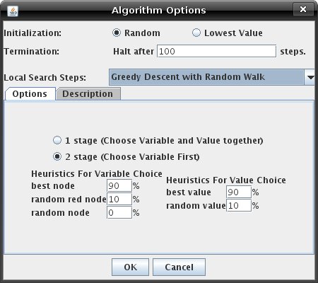
Tutorial 4: Stochastic Local Search Algorithms

The SLS applet implements several Stochastic Local Search algorithms for solving CSPs. The algorithm to use while solving the CSP can be selected and the appropriate options for that algorithm set by opening the "Algorithm Options" dialog box by clicking on "Algorithm Options..." under the "Hill Options" menu. The dialog box will look like the picture below:

Before you begin solving a CSP in this applet, the CSP must be initialized. This means that a value must be assigned to each variable in the CSP from its domain. The assignment can be done randomly or by lowest value by selecting the appropriate radio button next to "Initialization:".

The SLS applet attempts to find a solution to the CSP in a specified number of steps using the local search algorithm. If a solution hasn't been found by the specified number of steps, the searching halts. This number can be specified in the field next to "Termination:". The default number of steps is 100.

Next to "Local Search Steps:" there is a drop down list of search algorithms from which you can select the desired search algorithm to use. For each algorithm selected, you can view a description of it by selecting the "Description" tab. Some of the algorithms also have options that you can set for the search, which can be specified under the "Options" tab.

Below is list of the available local search algorithms and a brief description of each:

Random Sampling

At each step this algorithm randomly creates a new solution. For each variable a new value is randomly chosen.

Random Walk

At each step this algorithm randomly chooses a new solution from the set of neighbouring solutions. The set of neighbouring solutions is defined in this applet as the solutions where a single variable has a different value.

Options: You may choose between a one or two stage heuristic. In the first case, the variable and value are chosen together; in the second case, the variable is chosen first and then the value.

Greedy Descent

At each step this algorithm chooses a value which improves the graph.

Options: You may choose between a one or two stage heuristic. In a one stage heuristic the variable and value are chosen together. In the two stage heuristic the variable is chosen first and then the value. The variable with the greatest number of conflicts in its edges is chosen and then the value which resolves the highest number of conflicts is chosen from this variable's set of values.

Greedy Descent with the Min Conflict Heuristic

The Min Conflict Heuristic is one of the first heuristics used for constraint satisfaction problems. (Minton et Al, 1992). It chooses a variable randomly from the set of variables with conflicts (red edges). The value which results in the fewest conflicts is chosen from the possible assignments for this variable. This heuristic is almost identical to Greedy Descent with Random Walk with a two stage heuristic choosing any red node 100% and best value 100%. The only difference is the MCH may return to the previous assignment.

Greedy Descent with Random Walk

At each step this algorithm probabilistically decides whether or not to take a greedy step (change to the best neighbour) or to take a random walk (change to any neighbour)

Options: You may choose between a one or two stage heuristic.  In the first case, the variable and value are chosen together; in the second case, the variable is chosen first and then the value. To increase the random walk percentage increase the "random ..." values.

Greedy Descent with Random Restart

This algorithm proceeds like the Greedy Descent algorithm but resets the variables to a new random solution at regular intervals.

Options: Reset Graph specifies the number of steps between random resets of the graph.

Greedy Descent with all Options

This algorithm provides all the options associated with Random Resets, Random Walk and Greedy Descent enabling free experimentation with these algorithms.

Simulated Annealing

Simulated annealing performs random guesses in the set of neighbours. If the temperature is very high it accepts most of the guesses irrespective of how much "better" they are than the current value. The temperature is decreased according to a schedule. As the temperature decreases the chance of accepting a guess which does not improve the solution decreases.

Options:

• Starting Temperature: the initial temperature at which the search begins. A higher temperature means that more guesses will be accepted. A temperature of 0 means that only guesses which decrease the cost function will be accepted.
• Boltzman Constant (K) : A constant which is multiplied by the temperature when the probability of accepting a guess must be determined. P(accepting guess) = exp( -dE/ KT ) where dE is a measure of how much this guess would improve the solution.
• Descent Function: Determines how the temperature is decreased.
• Constant: it stays at the Starting Temperature.
• Linear: it decreases by the value of the Descent Rate each adjustment. New T = Old T - Descent Rate
• Logarithmic: it decreases by a factor of the Descent Rate each adjustment. New T = Old T x (1 - Descent Rate)
• Descent Rate: Determines how large each adjustment is. Is used differently by different descent functions.
• Maintain Temperature: Determines how many guesses the temperature will remain constant before it is adjusted.